- I decided to study deep learning and read a book on deep learning [1].
- Furthermore, I created a handwritten digit recognition program using the MNIST dataset [2]
- MNIST is like the Hello World for building classifiers
- I’ll use the simplest feedforward neural network (FFNN) (I don’t understand the others well)
- Just reading chapters 1 through 4 provides enough information for implementation
- Composed of only 3 layers: input layer, hidden layer, and output layer
- I’ll use existing packages for matrix calculations and datasets
- I’ll implement the image recognition program itself (not using caffe, TensorFlow, etc.)
- It seems Python is standard in this field, so I’ll follow that
- However, I’m postponing Jupyter (IPython) as the setup was troublesome
- All source code is available at [3]
Building the Feedforward Neural Network
-
Adopting a feedforward neural network (FFNN) with a simple structure
- Also called multilayer perceptron
-
Classify input data into multiple classes
-
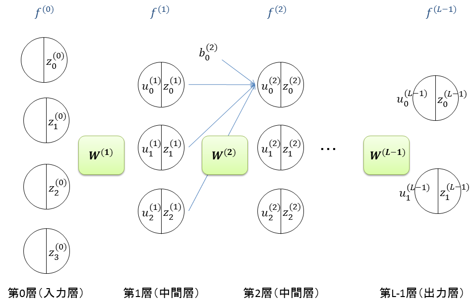
Build the network as shown in the figure
- \(L\): Number of layers. Three layers are sufficient: input layer, hidden layer, and output layer
- \(f^{(l)}(u)\): Activation function at layer \(l\)
- \(f^{(l)}(u) = \frac{1}{1+e^{-u}} \): For layers other than the output layer, use the logistic function
- \(u_i^{(l)}\): Input to the \(i\)-th unit in layer \(l\)
- \(z_{i}^{(l)}=f^{(l)}(u_i^{(l)})\): Output from the \(i\)-th unit in layer \(l\)
- \(\mathbf{W}^{(l)}\): Weight matrix between layer \(l-1\) and layer \(l\)
-
Represent input/output of each layer as column vectors
- \(\mathbf{u^{(l)}} = [u_0^{(l)} u_1^{(l)} \dots u_i^{(l)} \dots]^{T}\): Column vector representing inputs to units in layer \(l\)
- \(\mathbf{z^{(l)}} = [z_0^{(l)} z_1^{(l)} \dots z_i^{(l)} \dots]^{T}\): Column vector representing outputs from units in layer \(l\)
-
At this time, forward propagation (input layer->hidden layer->output layer) can be written with matrix operations
- Given input as column vector \(\mathbf{x}\), \(\mathbf{z}^{(0)} = \mathbf{x}\)
- Given output as column vector \(\mathbf{y}\), \(\mathbf{y} = \mathbf{z}^{(L-1)}\)
- \(\mathbf{u^{(l+1)}} = \mathbf{W}^{(l+1)} \mathbf{z}^{(l)} + \mathbf{b}^{(l+1)}\)
- \(\mathbf{z^{(l+1)}} = f^{(l+1)}(\mathbf{u^{(l+1)}})\)
- Where \(\mathbf{b}^{(l)}\) is the bias of layer \(l\)
-
If just classifying, we’re done here. \(\mathbf{y}\) is the classification result.
-
In the learning phase, we next perform backward propagation (output layer->hidden layer->input layer).
- \(\mathbf{d}\): Correct data for \(\mathbf{x}\)
- \(\mathbf{\Delta}^{(L-1)} = \mathbf{z}^{(L-1)} - \mathbf{d}\)
- \(\mathbf{\Delta}^{(l)} = f^{(l)’} ( \mathbf{u^{(l)}} ) \odot \mathbf{W}^{(l+1)T} \mathbf{\Delta}^{(l+1)} \)
- \(\odot\): Element-wise product of matrices
- \(f^{(l)’}(u)\): Derivative of \(f^{(l)}(u)\)
-
Once \(\mathbf{\Delta}^{(l)}\) is obtained, update weights and biases based on it.
- \(\mathbf{W}^{(l)} \leftarrow \mathbf{W}^{(l)} - \epsilon \mathbf{\Delta^{(l)}} \mathbf{z}^{(l-1)T} \)
- \(\mathbf{b}^{(l)} \leftarrow \mathbf{b}^{(l)} - \epsilon \mathbf{\Delta^{(l)}} [1 1 \dots 1]^T \)
- \(\epsilon\): Learning rate.
-
I wonder if determining the learning rate, initial weight values, number of units, and number of training epochs is based on rules of thumb
-
It seems efficient for parallelization to pass multiple training data (mini-batch) simultaneously, so the program below uses mini-batches
# Apply logistic() to each element of the matrix
def logistic(U):
    return 1.0/(1.0 + np.exp(-1.0*U))

# Apply logistic_deriv() to each element of the matrix
def logistic_deriv(U):
    t = logistic(U)
    return t * (1.0-t)

def softmax(U):
    U = U - np.max(U, axis=0) # Normalize U
    U = np.exp(U)             # Apply exp() to all elements
    U = U / np.sum(U, axis=0)
    return U

# Multilayer network, multiclass classifier
class FeedforwardNeuralNetwork:

    # Constructor
    # sizes: Number of units in input layer, hidden layer, output layer
    # f: Activation function. Not needed for input layer
    # f_deriv: Only for hidden layers
    def __init__(self, sizes, f, f_deriv):

        # Number of units in each layer
        self.sizes = sizes

        # Number of layers
        self.L = len(sizes)

        # Activation function f, derivative of activation function f_deriv
        self.f, self.f_deriv = f, f_deriv

        # Weights W and biases b for each layer
        self.W, self.b = list(range(self.L)), list(range(self.L))
        for l in range(1,self.L):
            self.W[l]       = np.random.uniform(-1.0,1.0,(sizes[l], sizes[l-1]))
            self.b[l]       = np.random.uniform(-1.0,1.0,(sizes[l], 1))

    # Propagate data through the network
    #
    # X=[x1,x2,...xn]: Input data (mini-batch), each data xi is a column vector
    # D=[y1,y2....yn]: Correct output corresponding to X
    #
    # D==[]: Predict by forward propagation. Return value is output corresponding to X.
    # D!=[]: Learn weights by forward and backward propagation. Return value is error.
    def propagate(self, X, D = []):
        # --- Forward propagation ---
        N = len(X[0]) # Number of columns
        Z, U = list(range(self.L)), list(range(self.L))
        Z[0] = np.array(X,dtype=np.float64)
        for l in range(1,self.L):
            U[l] = np.dot(self.W[l],Z[l-1]) + np.dot(self.b[l],np.ones((1,N)))
            U[l] = U[l].astype(np.float64)
            Z[l] = self.f[l]( U[l] )
        if len(D)==0:
            return Z[self.L-1]

        # --- Backward propagation ---
        De = list(range(self.L))
        Y  = Z[ self.L -1]
        D  = np.array(D)
        eps = 0.4 # Learning rate

        # Calculate De
        De[ self.L-1 ] = Y - D # Note. Different from P51. Looking at P49, this seems correct?
        for l in range(self.L-2,0,-1):
            De[l] = self.f_deriv[l]( U[l] ) * np.dot(self.W[l+1].T , De[l+1] )

        # Update W, b
        for l in range(self.L-1,0,-1):
            self.W[l] = self.W[l] -  eps/N*np.dot(De[l] , Z[l-1].T)
            self.b[l] = self.b[l] -  eps/N*np.dot(De[l] , np.ones((N, 1)))

        # Return error
        return np.power(De[self.L-1],2).sum()/N
Verification
- Let’s have the network convert 3-bit binary numbers to 1-digit decimal numbers
- Like 110 -> 6
# Return the index corresponding to the largest number in list li
# l2n( [00 11 27 19 18] ) -> 2
def l2n(li):
    return max(range(len(li)), key=(lambda i: li[i]))

# Convert number x to a list of size 10
# n2l(3) -> [0 0 0 1 0 0 0 0 0 0]
def n2l(x):
    res = [0,0,0,0,0,0,0,0,0,0]
    res[x] = 1
    return res

# Verification of FeedforwardNeuralNetwork operation with binary to decimal conversion
def binary2decimal_test():
    dl = FeedforwardNeuralNetwork(
            [3,8,10], [None,logistic,softmax], [None,logistic_deriv,None])
    for i in range(1000):
        dl.propagate(
                [[0,1,0,1,0,1,0,1], # Training data (input)
                 [0,0,1,1,0,0,1,1],
                 [0,0,0,0,1,1,1,1]],
                [[1,0,0,0,0,0,0,0], # Training data (correct answer)
                 [0,1,0,0,0,0,0,0],
                 [0,0,1,0,0,0,0,0],
                 [0,0,0,1,0,0,0,0],
                 [0,0,0,0,1,0,0,0],
                 [0,0,0,0,0,1,0,0],
                 [0,0,0,0,0,0,1,0],
                 [0,0,0,0,0,0,0,1],
                 [0,0,0,0,0,0,0,0],
                 [0,0,0,0,0,0,0,0]])
    X = [[0], # Test data
         [1],
         [1]]
    Y = dl.propagate(X)
    print("input:")
    for i in range(2,-1,-1):
        print(X[i][0], end='')
    print("\nanswer:")
    for i in range(10):
        print(str(i) + ": " + str(int(Y[i][0]*100)) + "%")

binary2decimal_test()
- Output results shown below.
- Binary 110 is successfully predicted as decimal 6.
input:
110
answer:
0: 0%
1: 0%
2: 1%
3: 0%
4: 1%
5: 0%
6: 95%
7: 1%
8: 0%
9: 0%
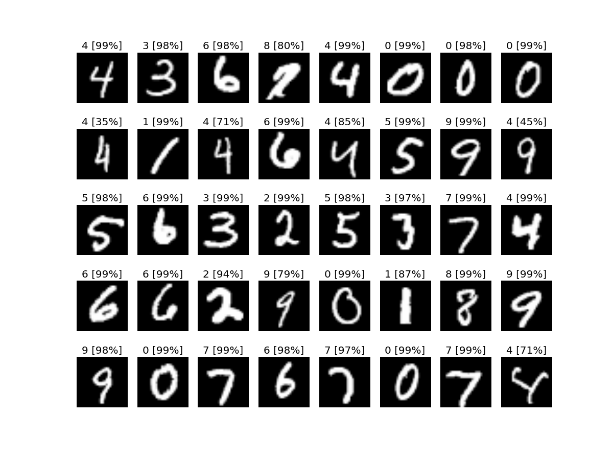
MNIST Image Recognition
- MNIST is a dataset of 70,000 handwritten digit images, each 28x28 pixels
- Python has fetch_mldata which automatically fetches MNIST data. Convenient.
- There are 70,000 images in total: 63,000 for training data, 7,000 for test data
- Data is normalized in advance to the range 0.0 to 1.0
- Learning rate is 0.4 (determined arbitrarily by parameter sweep)
- Initial weight values uniformly random in [-1 1]
- Number of units in input layer, hidden layer, output layer are 28x28, 100, 10 respectively (determined arbitrarily by parameter sweep)
# MNIST classifier
class MNIST:

    # Constructor
    def __init__(self):
        # MNIST dataset
        mnist = fetch_mldata('MNIST original', data_home=".")

        # Image data X, correct data y
        X = mnist.data
        y = mnist.target

        # Normalize to 0.0 to 1.0
        X = X.astype(np.float64)
        X /= X.max()

        # Split X and y into training data and test data
        # test_size: Proportion of test data
        self.X_train,self.X_test,self.y_train,self.y_test=train_test_split(X,y,test_size=0.1)

        # Build network
        self.dl = FeedforwardNeuralNetwork([28*28,100,10],
            [None,logistic,softmax], [None,logistic_deriv,None])

    # Train the network
    # num: Number of training iterations
    def learn(self, num):

        # Index set of training data
        train_indexes = list(range(0, self.X_train.shape[0]))

        for k in range(num):

            # Select mini-batch (learning unit)
            minibatch = np.random.choice(train_indexes, 50)

            # Extract training data and correct data according to mini-batch
            inputs  = []
            outputs = []
            for ix in minibatch:
                inputs.append(self.X_train[ix])
                outputs.append(n2l(int(self.y_train[ix])))
            inputs = np.array(inputs).T
            outputs = np.array(outputs).T

            # Learn
            self.dl.propagate(inputs, outputs)

            # Output progress
            if k% (num//100) ==0:
                if (k*100//num) % 10 ==0:
                    sys.stdout.write(str(k*100//num))
                else:
                    sys.stdout.write(".")
            sys.stdout.flush()
        print()

    # Classify data at index ix
    # ix: Index in test data
    def predict_one(self, ix):
        # Execute multiclass classification
        inputs = np.array([self.X_test[ix]]).T
        self.dl.propagate(inputs)

        # Output classifier results
        print("answer:")
        for i in range(10):
            print(str(i) + ": " + str(int(t[i][0]*100)) + "%")

        # Output image
        self.show_image(self.X_test[ix])

    # Test all test data and output precision, recall, F-value
    def predict_all(self):
        # Execute multiclass classification
        predictions = self.dl.propagate(np.array(self.X_test).T)

        # Format
        predictions = np.array(list(map(l2n, predictions.T)))

        # Output precision, recall, F-value
        print(classification_report(self.y_test, predictions))

a = MNIST()

print("start learning")
a.learn(2000)

print("start testing")
a.predict_all()
- Results are as follows
- Precision, recall, and F1-score are each 93%
- Fairly good accuracy for something made by trial and error?
- Not sure how it is in absolute terms
$ python3 main.py
start learning
0.........10.........20.........30.........40.........50.........60.........70.........80.........90.........
start testing
             precision    recall  f1-score   support

        0.0       0.96      0.97      0.96       682
        1.0       0.95      0.98      0.97       740
        2.0       0.94      0.88      0.91       721
        3.0       0.93      0.93      0.93       706
        4.0       0.92      0.93      0.92       720
        5.0       0.93      0.90      0.91       627
        6.0       0.93      0.95      0.94       680
        7.0       0.93      0.93      0.93       712
        8.0       0.88      0.93      0.91       702
        9.0       0.93      0.88      0.90       710

avg / total       0.93      0.93      0.93      7000
Future Work
I’ll look at the following topics:
- Autoencoder: Update weights through unsupervised learning to make output close to input
- Convolutional Neural Network (CNN): Major in image processing
- Recurrent Neural Network (RNN): Major in speech recognition and handwriting recognition
- Boltzmann Machine: Operates probabilistically (I don’t understand it well)
References
- [1] Takayuki Okatani, Deep Learning (Machine Learning Professional Series), http://goo.gl/c0MV0f
- [2] THE MNIST DATABASE of handwritten digits, http://yann.lecun.com/exdb/mnist/
- [3] https://github.com/bobuhiro11/ffnn/blob/master/main.py