- For simplicity, consider a one-dimensional wave
- Let the value at coordinate \(x\) at time \(t\) be \(f(x-ut)\)
- For example, if a sine wave moves in the positive x-axis direction at velocity \(u\), then \(f(x-ut) = sin(x-ut)\)
- At this time, \(\frac{\partial f}{\partial t} + u \frac{\partial f}{\partial x} =0 \) holds. This is the advection equation
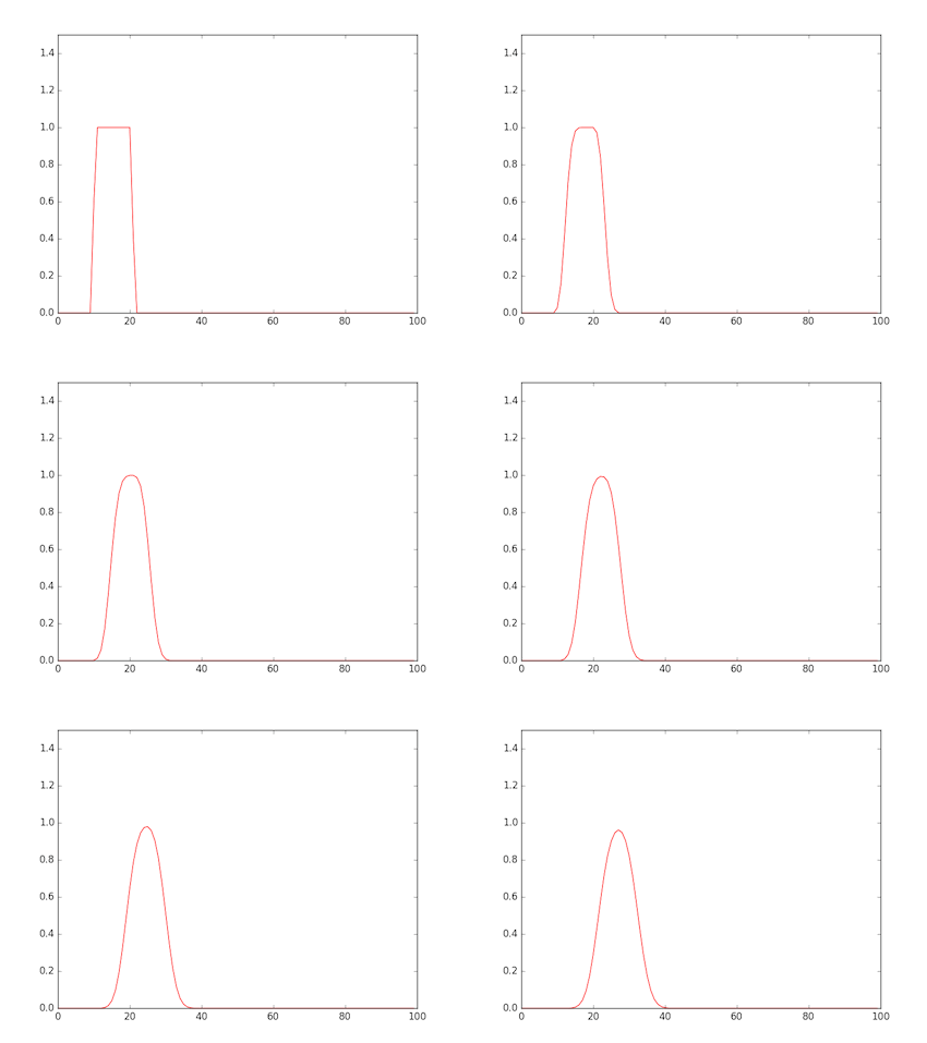
First-Order Upwind Difference Method#
- Approximate with a straight line
- Since this is numerical analysis, \(x\) is discrete like \(\dots,x_{i-1},x_i,x_{i+1},\dots\)
- Let the approximation of \(f\) at \(x = x_i\) be \(F_i^n(x)\)
- This method approximates with a straight line, so \(F_i^n(x)=a(x-x_i) + f_i^n, a = \frac{f_i^n - f_{i-1}^n}{\Delta x}\)
- Where \(f_i^n\) is the value after advancing the time step \(n\) times at \(x = x_i\)
- Time advances by \(\Delta t\) per time step
- When advancing the time step, $f_i^{n+1} = F_i^n(x_i-u\Delta t) = a(-u \Delta t) + f_i^n= - \frac{u \Delta t}{\Delta x}(f_i^n - f_{i-1}^n) + f_i^n$
- In the program, just repeat the following with $K=u \frac{\Delta t}{\Delta x}$
- The figure shows a rectangular wave input
- There’s also downwind
for(i=1; i<99; i++) f_new[i] = -K * (f[i]-f[i-1]) + f[i];
for(i=1; i<99; i++) f[i] = f_new[i];

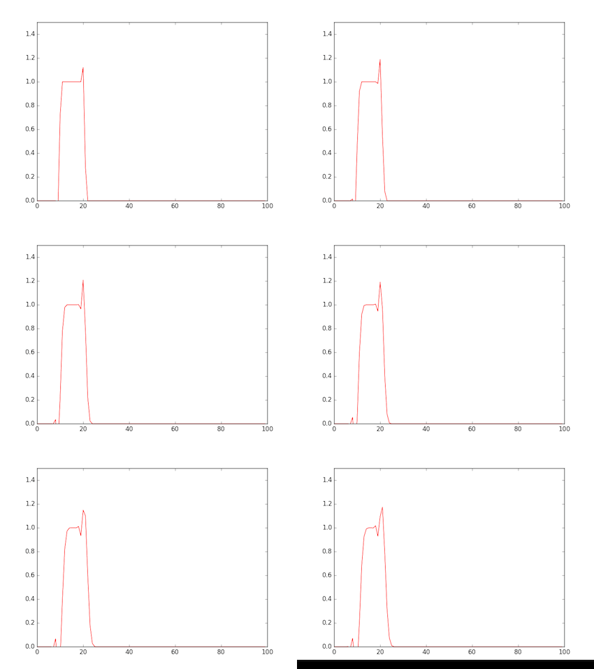
Lax-Wendroff Method#
- Approximate with a quadratic function
- Approximate with $F_i^n(x) = a(x-x_i)^2 + b(x-x_i) + c$
- Since three constants $a,b,c$ are needed, put appropriate values into $x$:
- $F_i^n(x_{i-1}) = a \Delta x ^2 - b \Delta x + c = f_{i-1}^n$
- $F_i^n(x_{i}) = c = f_{i-1}^n$
- $F_i^n(x_{i+1}) = a \Delta x ^2 + b \Delta x + c = f_{i+1}^n$
- Where $x_{i+1} - x_{i} = x_{i} - x_{i-1}=\Delta x$
- Solving this gives:
$$
F_{i}^n(x) = a(x-x_i)^2 + b(x-x_i) + f_i^n, \\
a = \frac{f_{i+1}^n - 2f_{i}^n + f_{i-1}^n}{2\Delta x^2},
b = \frac{f_{i+1}^n - f_{i-1}^n}{2\Delta x}
$$
- When advancing the time step:
$$
f_i^{n+1} = F_i^n(x_i-u\Delta t) = f_i^n - \frac{u\Delta t}{2 \Delta x}(f_{i+1}^n - f_{i-1}^n) + \frac{(u\Delta t)^2}{2 \Delta x ^2}(f_{i+1}^n -2 f_i^n- f_{i-1}^n)
$$
- In the program, similar to upwind difference, just repeat the following with $K=u \frac{\Delta t}{\Delta x}$
for(i=1; i<99; i++) f_new[i] = f[i] - K*K*(f[i+1]-f[i-1])/2.0 + K*K*(f[i+1]-2*f[i]+f[i-1])/2.0;
for(i=1; i<99; i++) f[i] = f_new[i];

CIP Method#
- In addition to the function itself, advect its derivative and approximate with a cubic function
- First, differentiate the advection equation $\frac{\partial f}{\partial t} + u \frac{\partial f}{\partial x} = 0$ with respect to $x$
- $\frac{\partial g}{\partial t} + u \frac{\partial g}{\partial x} = -g \frac{\partial u}{\partial x}$
- Next, approximate $f$ with $F_i^n(x) = a(x-x_i)^3 + b(x-x_i)^2 c(x-x_i) + d$
- Also differentiate $F_i^n(x)$ with respect to $x$:
- $\frac{d F_i^n(x)}{dx} = 3a(x-x_i)^2 + 2b(x-x_i) + c$
- Find the four constants $a,b,c,d$ appropriately:
- $F_i^n(x_i) = d = f_i^n$
- $\frac{d F_i^n(x_i)}{dx} = c = g_i^n$
- $F_i^n(x_{i-1}) = -a \Delta x^3+b \Delta x^2 - c \Delta x + d = f_{i-1}^n$
- $\frac{d F_i^n(x_{i-1})}{dx} = 3a \Delta x^2 - 2b \Delta x + c = g_{i-1}^n$
- Solving this gives:
$$
a = \frac{g_i^n + g_{i-1}^n}{\Delta x^2} - \frac{2 (f_i^n - f_{i-1}^n)}{\Delta x^3},
b = \frac{3(f_{i-1}^n + f_{i}^n)}{\Delta x^2} - \frac{2 g_i^n + g_{i-1}^n }{\Delta x} \\
$$
- When advancing the time step:
$$
f_i^{n+1} = F_i^n(x_i-u\Delta t) = -a u^3 \Delta t^3 + b u^2 \Delta t ^2 -c u \Delta t + d, \\
g_i^{n+1} = \frac{F_i^n}{dx}(x_i-u\Delta t) = 3a (-u \Delta t)^2 + 2b(-u \Delta t) +c
$$
dx = 1.0;      // dx
d  = -dx;      // -dx
gzi = -dx * K; // -dx * u * dt/dx = -u*dt
for(i=1; i<99; i++){
    a = (g[i] + g[i-1]) / (d*d) + 2.0 * (f[i]-f[i-1])/(d*d*d);
    b = 3.0 * (f[i-1]-f[i])/(d*d) - (2.0*g[i]+g[i-1])/d;
    f_new[i] = ((a*gzi+b)*gzi+g[i])*gzi+f[i];
    g_new[i] = (3.0*a*gzi+2.0*b)*gzi++g[i];
}
for(i=1; i<99; i++){
    f[i] = f_new[i];
    g[i] = g_new[i];
}

References#


